Introduction
Goals of the Query UI
This tool will help you translate your research questions into Timur queries, which you can run in your browser to generate a data frame. Most research questions begin with a root question and a set of desired data points, as well as some filtering criteria. For example, "I’m curious about patients with positive disease status, under the age of 50. In particular, I also want to know their sex at birth and IL-6 levels." Once you receive a data frame with this information, you can then run various analyses on your own computer to explore relationships among the data. In this document we’ll discuss:
-
The thought process behind converting your research question into a question that fits the Timur models.
How to input that question into the Query UI.
-
How to make sure you have a "flat" data frame, which will make your subsequent analyses simpler.
We’ll start with showing how to use the Map view to understand a project’s models, walk through the overall Query UI, and then step through some concrete examples, showing how to get from a research question to a data frame.
Map and Model Overview
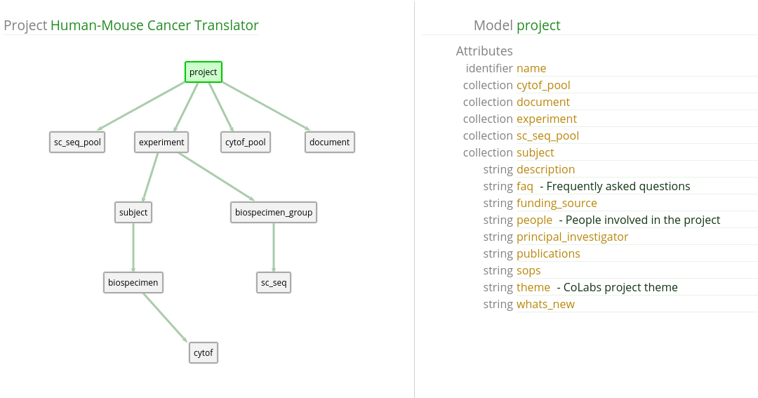
The Timur Map view is available by clicking on the Map link in the top navigation bar, once you navigate to your project.
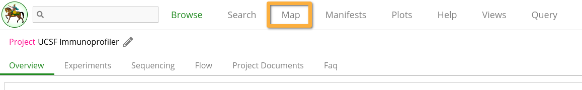
Clicking that brings up a view with a graphical representation of the project models, as well as a tabular listing of the selected model’s attributes. By default the project model is selected.
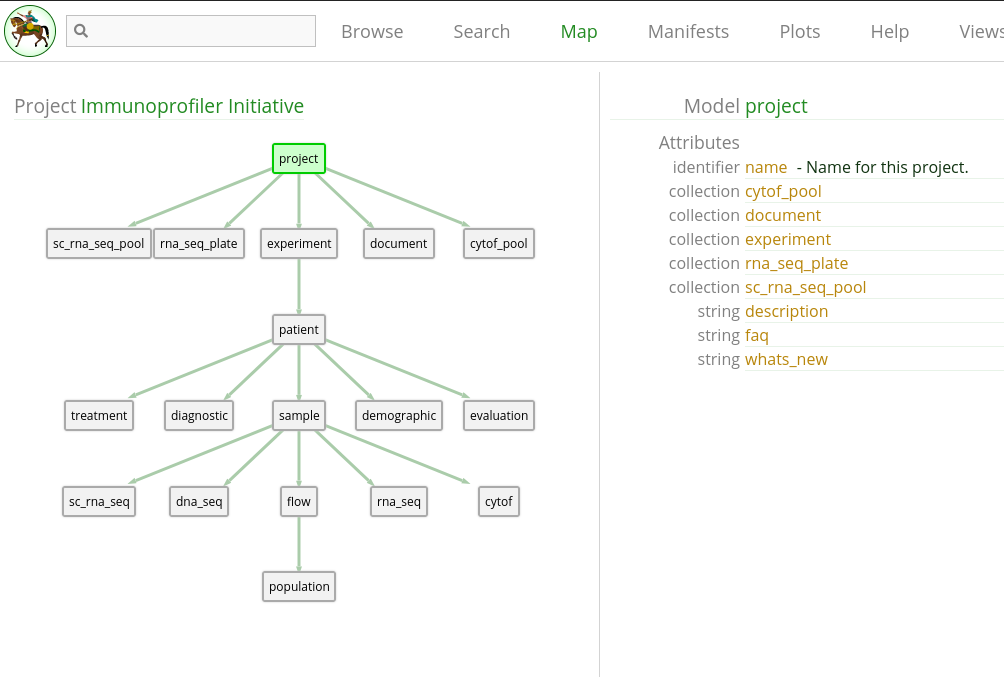
We won’t describe the entire Map view here, only the relevant portions to constructing queries. Each box in the map represents a specific model, and each attribute represents some aspect of that model. You can think of a model as a high-level concept (i.e. Bulk RNA sequencing), and the attributes as specific details within that concept (i.e. Eisenberg score). Within the Timur database, each model contains individual records that are concrete data points identified by unique identifier strings, such as an individual library of RNASeq or tube of CyTOF.
Paths Between Models
Often in this document we will discuss paths between models, and intervening models that appear along this path. When you specify a filter or column, the Query UI will attempt to find the shortest path between the root model and your filter or column model – shortest path meaning the fewest number of intervening models between the starting point and the destination. You can see the paths on the map, and while you do not have to select the path yourself, you will want to note the intervening models, because they may affect how you toggle the filter and column settings in your query.
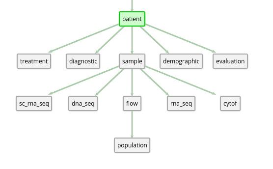
Let’s look at 1.3, where we can use the Patient subtree for some examples. If your root model is Patient, and you want to add a filter based on some Flow attribute, the path would be Patient -> Sample -> Flow. If your root model is RnaSeq, and you want to filter based on some Demographic value, the path in that case is RnaSeq -> Sample -> Patient -> Demographic. Links are non-parent-child relationships between models, and you can find them by viewing the attributes for a model (links currently do not appear visually on the graph). Paths may also traverse through these links, if they provide a shorter path between two models.
Travel Directionality
You’ll notice that the visual representation of the map looks like a tree, with the project at the top of the tree. We’ll thus frequently use the terms "up the tree" and "down the tree" to describe relationships between models. This directionality will be important to understand if the relationship is one-to-one or one-to-many, which affects the shape of your final data frame.
Up the tree
The way models are designed, all relationships that go "up the tree" are one-to-one relationships. When doing queries, one-to-one relationships result in a single data point inside of a data frame cell, which makes analysis simpler.
For example, looking at 1.2, we can see that Patient is above Sample in the tree. So going from Sample to Patient means we’re moving up the tree – and each Sample belongs to one and only one Patient. In a data frame, this might look like 1.1.
| Sample | Patient |
|---|---|
| Patient001.T1 | Patient001 |
| Patient001.N1 | Patient001 |
| Patient002.T1 | Patient002 |
| Patient003.N1 | Patient003 |
Note that knowing the relationship "up the tree" gives us no information about the inverse direction, down the tree. To determine the relationship type going down the tree, we’ll need to inspect the attributes.
Down the tree
Most relationships that are "down the tree" are one-to-many, which can result in data frames with nested information. If you take our previous example of Patients and Samples, we can look at the Patient attributes to see what kind of relationship exists between the two when going down the tree. This can be seen in 1.4.
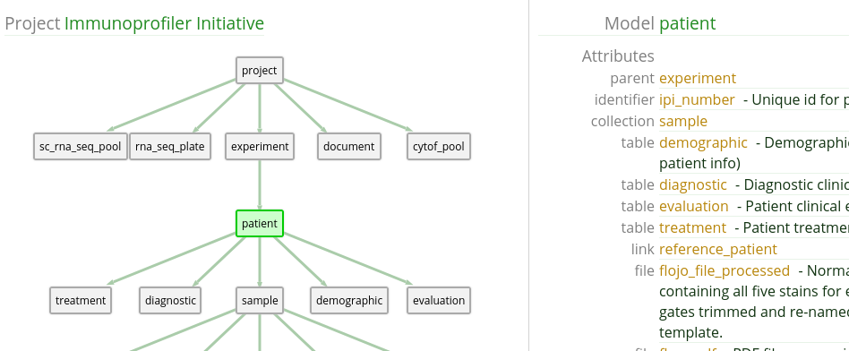
We see that Sample is a ‘collection‘ type attribute. This means that a single Patient has zero or more Samples. In a non-flat data frame, querying this out results in a nested data frame, like in 1.2.
| Patient | Sample |
|---|---|
| Patient001 | Patient001.T1, Patient001.N1 |
| Patient002 | Patient002.T1 |
| Patient003 | Patient003.N1 |
To analyze a nested data frame like this, you would have to extract the nested data yourself. To get a flat data frame, you can either restructure your query to take advantage of up the tree relationships, or use column slicing and extract only the data values you are interested in.
For one-to-one "down the tree" relationships (they are rare, but do exist in several projects), you do not have to worry about nested data.
Query UI Overview
The Timur Query UI is available by clicking on the Query link in the top navigation bar, once you navigate to your project.
Clicking that brings up an empty form builder, with a selector for a "Root Model".
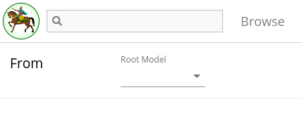
Once you select a root model, the rest of the form builder appears.
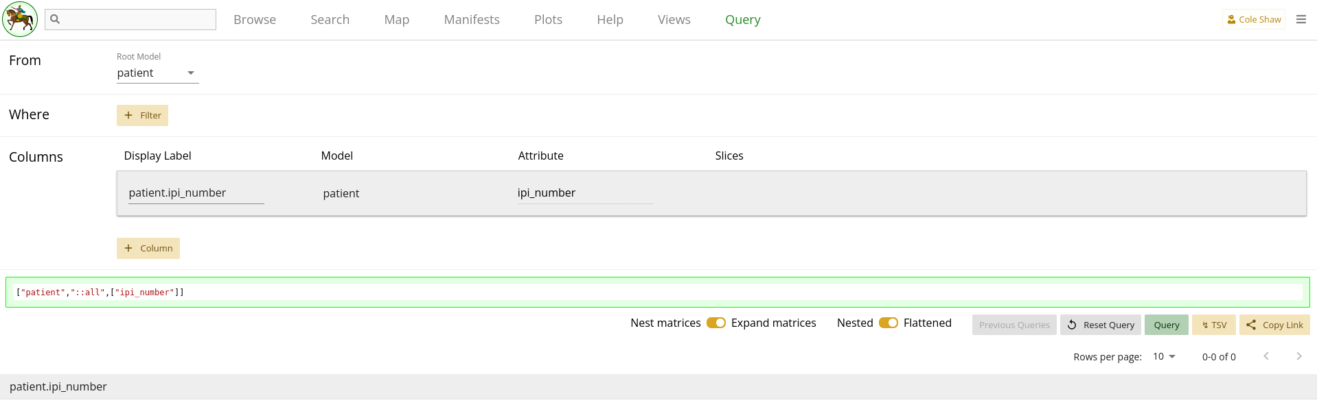
Root Model
The root model forms the starting point of your query. The identifier of the model is the left-most column of your data frame and acts as the unique identifier for the output. Generally, it is the starting point of the question you’ve formulated. For example, if you want to know "All the patients that are COVID positive and their IL-6 levels", you would most likely want to start with Patient as your root model. We will explore a couple different ways to extract the same data with different root models, but we’ll start with this more straightforward approach in each example.
Note that once you select a root model, its identifier is automatically added as a column and appears in the output data frame. Unlike other columns which you will add later, this column can only be removed by selecting a different root model.
Where Filters
Most research questions have some sort of constraint on the data that you want to analyze. You can think of Where Filters as applying those constraints and limiting the rows that appear in your data frame. This section of the form builder allows you to specify the set of filters that will narrow down the returned data.
As an added bonus, remember that where filters are one way that we might be able to narrow down a nested data frame into a flat data frame.
Specifying a filter
To specify a filter, you will need three or four basic pieces of information:
The model you want to filter on.
-
Clauses that you want to apply to the filter model or its children models. Each clause is composed of:
(sometimes) An "Any" or "Every" statement.
The clause model (can be same as the filter model).
The clause model’s attribute you want to filter on.
The operator you want to apply.
(sometimes) The operand to evaluate the operator against.
For example, if you wanted to filter on Patients with age greater than 50, you would need to know that "age" in IPI is contained in the demographic table. Note that only models that have a valid path from your root model will appear in the filter’s Model selector.
Once you have selected a filter model, you will need to add one or more
clauses to your filter. A clause is a condition on a specific model – either
the filter model itself, or a child of the filter model. If the clause model
has a one-to-many relationship with the filter model, you will also be able to
select Any or Every as part of the condition.
Once you determine the right clause model, you’ll have to determine the attribute name. For non-table models, you can use the Map view to determine the attribute you want. For tables, you will have to inspect the table and find the right "Name" or "Value" that you want to filter on. The simplest way to do that is probably with the Search page, to view the raw table data.
One tricky operator to apply is Is present or
Is missing on models. When you want to know if an attribute on a
model is populated, you might specify a filter like "Samples where
tissue_type Is present", to mean "Sample records where the
tissue_type field has some data provided". When you attempt to do
the same with a "collection" type attribute (i.e. Samples with RnaSeq data),
you cannot do a "Samples where RnaSeq Is present" query, since
rna_seq will not appear as an attribute for Sample. Instead, you
have to add a filter like "RnaSeq where tube_name Is present",
using the identifier of the RnaSeq model.
If using the In or Not in operator, you have to
provide a comma-separated string with no spaces. i.e. if you want Patient IDs
in the set Patient 5, Patient 9, and Patient 11, you would construct the
operand as:
Patient5,Patient9,Patient11As you add and edit filters, you can see them appear in the query preview. While the exact syntax of that section may not be very intuitive (and that is okay!), hopefully as you edit the filters you can see how your filters affect the query and the output data frame.
You can check 3.1 for a list of operators for each type of attribute.
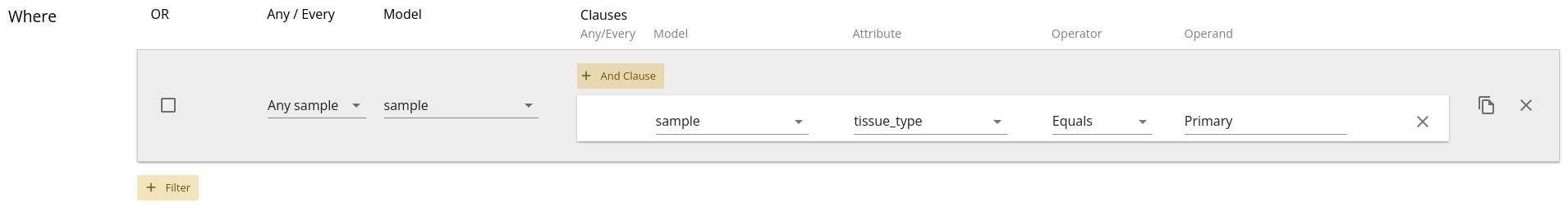
Any vs. Every
When filters traverse across models, any one-to-many relationship creates the
opportunity to also specify an "Any" or "Every" operator. These models are
calculated by the tool and will appear to the left of the filter model. For
example, when using the Patient as a root model, if we add in a Sample filter
to only return samples with tissue_type as "Primary" we’ll see a
selector appear with "Any Sample" or "Every Sample" as options. This is seen
in 1.8.
By default, "Any" is selected. This means that you want records where Any of the Samples meet the criteria. If a Patient has three Samples, one or more of them must be labelled as Primary in order for the Patient to be included in the output data frame. Only Patients with zero Primary Samples will be left out of the data set. If you select "Every", that means you expect every single Sample attached to that Patient to meet the criteria. So if a Patient has three Samples, all of them must be labelled as Primary for that Patient to be included in the output data frame. Patients with one or more non-Primary Samples will be left out of the data set.
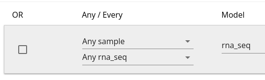
When you have multiple models in the path from your root model to the filter model, you will have an Any / Every toggle for each one-to-many relationship in the path, and each combination of selections will result in a different set of output data. An example is shown in 1.9, where Patient has a one-to-many relationship with Sample, and Sample has a one-to-many relationship with RnaSeq, and so two Any / Every toggles appear when you add an RnaSeq filter.
Note that the same Any / Every reasoning applies to the clauses within a given filter, so you can control how a clause affects the filter’s output using those selectors.
And and Or
Sometimes you may want to combine filters using AND or OR logic. For example, I want Patients who are older than 50 OR younger than 25 (or conversely, I want Patients who are younger than 50 AND older than 25). Currently, the Query UI supports a very simple version of this – if you need to construct more complicated queries, please let the Data Library Engineering team know, and we can add that ability as a feature request.
By default, all filters are applied as AND filters. However, the checkboxes on the left of each filter, as shown in 1.8, let you add one layer of OR filters. All checked filters are aggregated into a single OR statement that is then ANDed with the other filters.
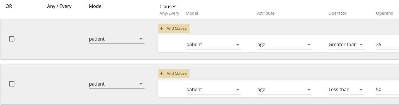
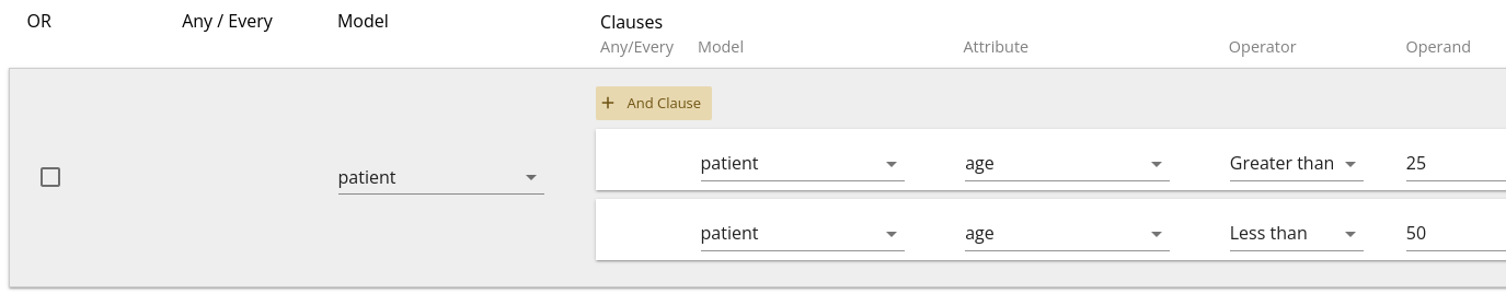
For example, a query with filters as shown in 1.10 would be translated as "Patients between the ages of 25 and 50".
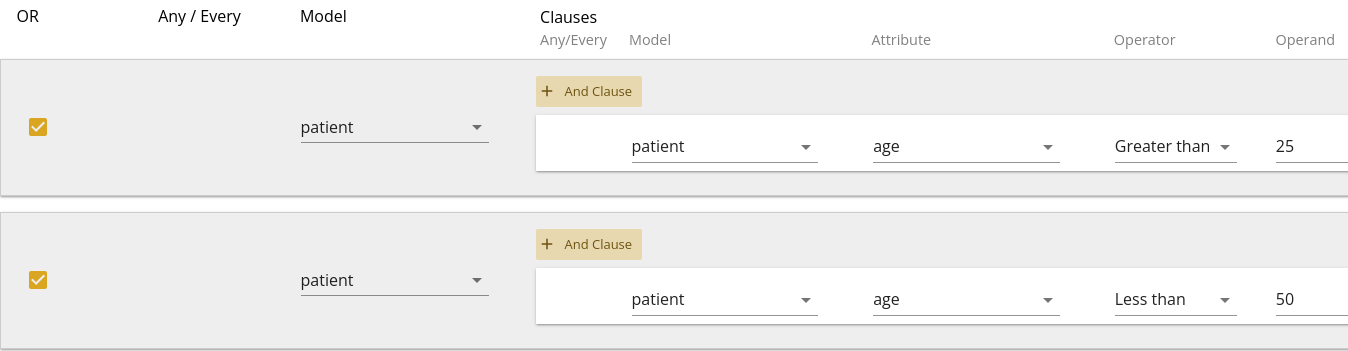
Whereas a query with filters as shown in 1.11 would be translated as "Patients older than 50 OR younger than 25".
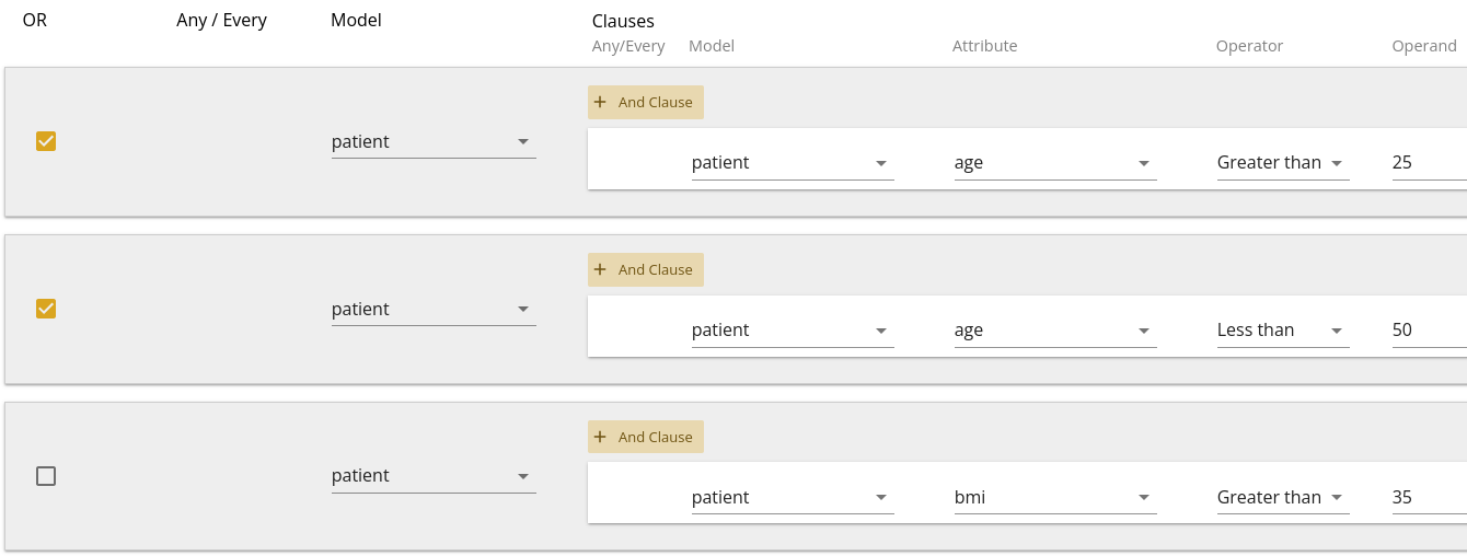
You can then combine these with other filters as shown in 1.12, which would be translated as "Patients older than 50 OR younger than 25, who have a bmi greater than 35".
Note that you can also combine "And"-type statements as multiple clauses on a single filter. Sometimes (especially with child-models), this is required to answer a specific question. The usage of multiple clauses versus multiple filters depends upon the question and in some cases, either may result in the same answer.
Columns
Where filters adjust which records of data to traverse, and thus affect the
contents of your data frame’s rows. But it takes more than rows to fill a data
frame. In the Columns section, you’ll pick what attributes to use to fill your
columns. This is the third section of the UI and appears auto-populated with
the identifier of your root model. You cannot directly remove this column, but
you can provide an alternate label to change how it appears in your data
frame. The default label is simply model_name.attribute_name.
Note that the columns are independent of the filters, so you can select columns on models that do not have filters.
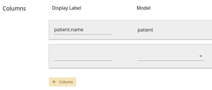
Specifying a Column
To specify a column, you only need the join model name and the attribute name:
The model you want data from.
The model’s attribute you want data for.
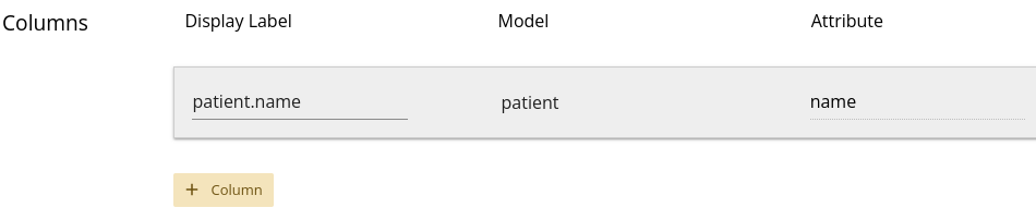
Note that the first input box for each column is for a
Display Label – this is optional, and it will default to
model_name.attribute_name if you leave the input blank.
Once you define the column’s model and attribute, it will appear in the data frame
at the bottom of the page. If you edit the Display Label for a
column, the data frame column heading should also change. You may need to do
this to prevent duplicate colum headings, which would confuse downstream R or
Python analysis.
As you add and edit columns and slices, you can also see them appear in the query preview. While the exact syntax of that section may not be very intuitive (and that is okay!), hopefully as you edit the columns and slices you can intuit how they affect the query and the output data frame.
Slicing
When your research question traverses across models that have one-to-many relationships, many times we are only interested in a subset of those relationships. In order to prevent nested data in your data frame, you can construct one or more Slices to select a subset of the nested data and get a flat data frame.
For example, you may only be interested in Tumor samples, in which case you might slice on the Patient -> Sample relationship. Column slicing gives you a subset of column data (as opposed to Filters, which give you a subset of row data). Going back to our example in 1.2 where Patient is one-to-many with Sample, we said that one way to construct a flat data frame with the same information was to use Sample as the root model. However, perhaps we are collecting additional data, and we really want to keep Patient as our root model. If we only want Tumor samples, we could construct a slice to select only the Tumor samples out of each Sample column, as in 1.17.

Assuming only a single tumor sample per patient, this would also result in a flat data frame. Slicing columns in this fashion is particularly helpful with clinical data, which generally appear in Timur as tables.
Note that slice construction requires the same set of information as a filter:
The model you want to filter on.
The model’s attribute you want to filter on.
The operator you want to apply.
(sometimes) The operand to evaluate the operator against.
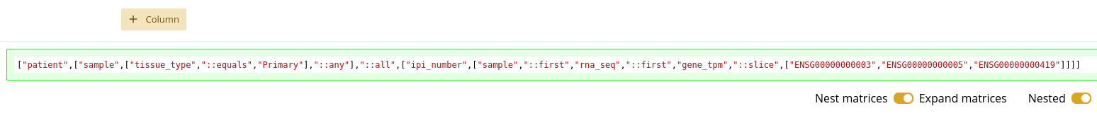
You can also slice out Matrix data, which is currently used for gene
expression and gene count data in the RnaSeq model. The main difference is
that the only slice operator in this case is Slice, and you then
provide a comma-separated list of Ensembl Gene Ids, with no spaces:
ENSG00000000003,ENSG00000000005,ENSG00000000419An example of a matrix slice can be seen in 1.18.

You can check 3.2 for a list of operators for each type of column slice attribute.
Query Preview
As you construct your query by adding filters and columns, there is a small text window that shows you what the raw Timur query will look like. It has a green outline, as seen in 1.19. While you should not expect to understand the exact syntax of this string, it should be helpful for you to see how changing the filters and columns changes this raw query. As you get more familiar with the Query UI, you may be able to intuit the kind of data in your data frame, based on this raw query string.
Data Frame
The bottom pane of the tool includes a set of control toggles and buttons as well as a data frame. While you contruct your query, the columns will appear in the data frame. This gives you an idea of what your final data will look like.

Reset query
If you would like to reset the entire query, you can click this button to remove all form entries and start over.
Query
Once you are satisfied with your data frame, you can click the
Query button at the top right of the data frame. Once data is
returned from the server, you will see it appear in the data frame. You can
navigate between pages or set a different number of items per page. Note that
setting a different number of items per page requires you to re-click the
Query button to re-fetch data.
Download TSV
To download all records in a tab-separated file, you can click the
Download TSV button. This will get you all records from the query
results. Note that with larger data frames or matrix data, the download may
take a while to complete.
Copy link
You can share and bookmark the query you’ve built, using the URL. For your convenience, clicking this button will put the entire URL into your clipboard, so you can paste it / share it with others. You can also bookmark the URL in your browser to save a specific query.
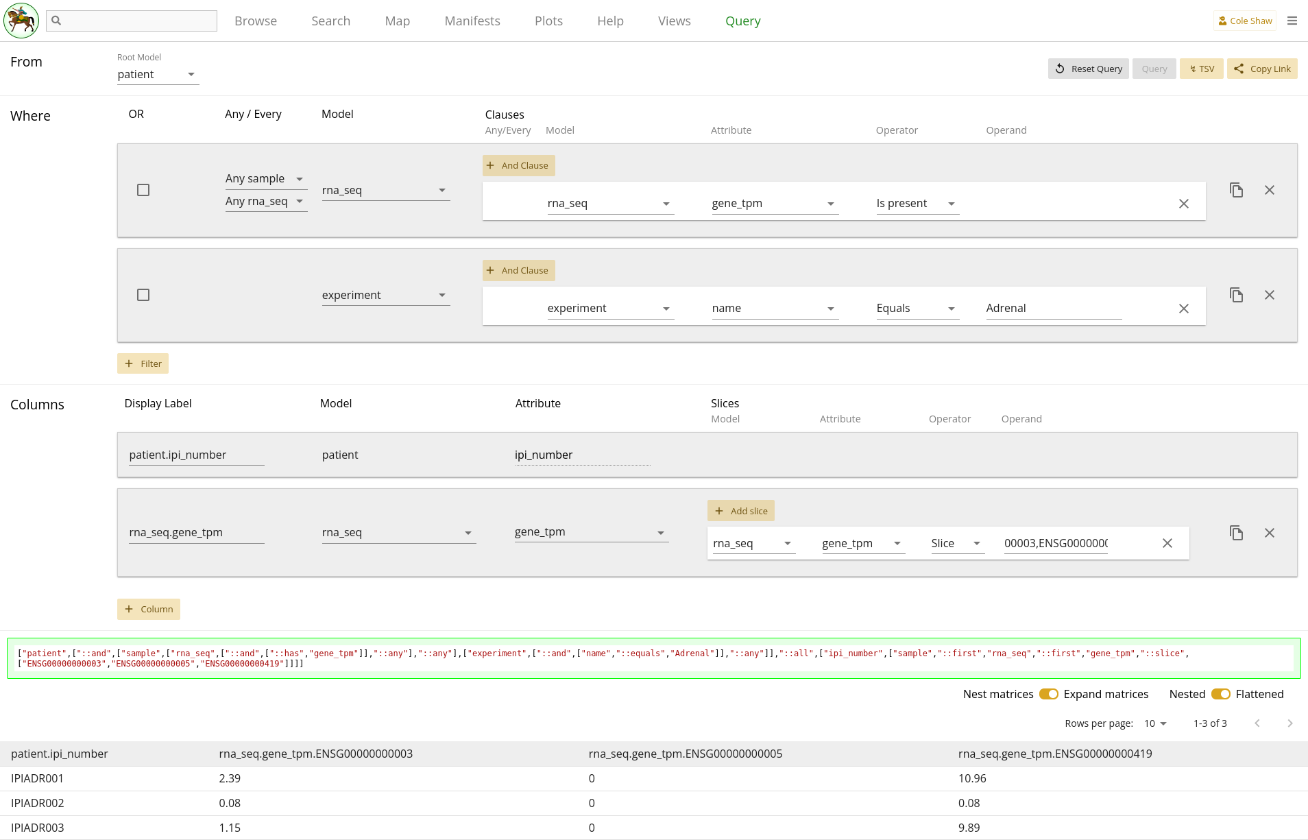
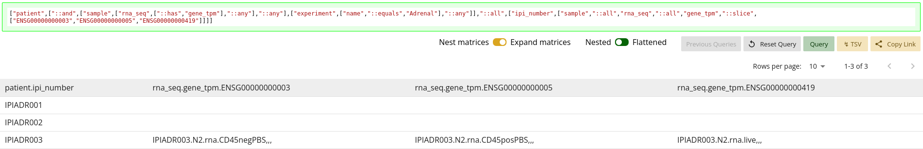
Nesting and Expanding Matrices
One thing you may have noticed from 1.21 is that we only specified two columns, but there are four columns in the data frame. This is because the default behavior of the tool is to expand matrix slices such that each data point is in its own, unique cell. This is generally more convenient for analysis.
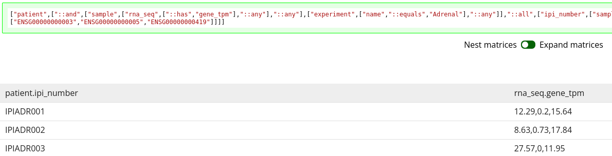
A toggle does exist for you to change that behavior. Toggling that to nested matrices results in the expected two columns, but leaves the matrix data all joined in a single cell, with no clear labelling of which data point belongs to which Ensembl gene code, as seen in 1.22.
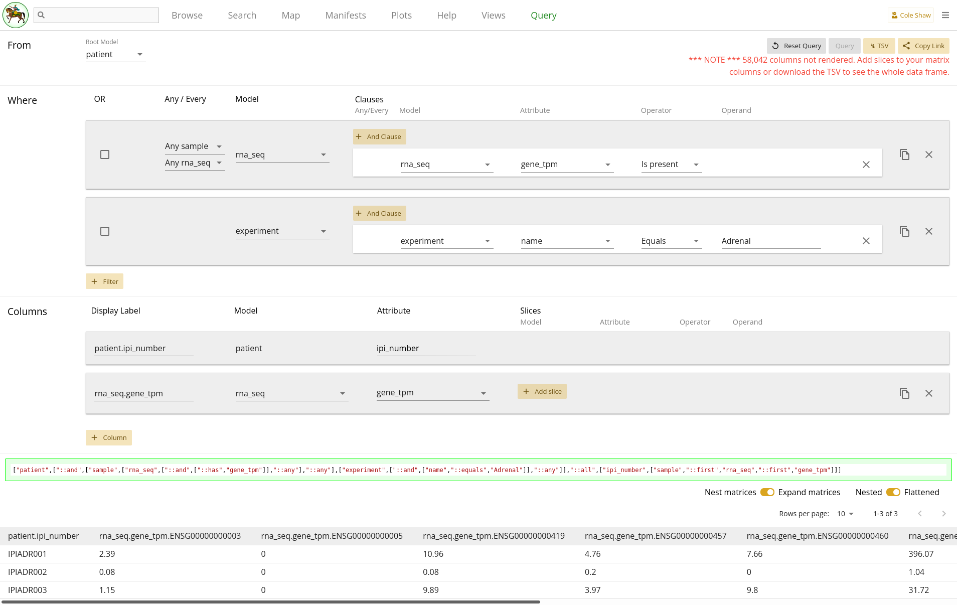
If you include a matrix attribute as a column but do not slice it, and if the
toggle is switched to Expand matrices, the UI will expand the
column with all possible gene codes. This results in over 58,000 columns! The
UI will only render a maximum of 10, and to see the entire data set, you will
have to download the TSV. You will see a warning for this, as seen in 1.23. Downloading this TSV may be a slow operation, since the TSV is generated in
your browser. If you need to download an entire gene expression matrix, the
Search page may offer faster performance, once you have identified the
rna_seq records you want to pull data for. Alternatively, you can
add a column slice to your query and specify just the genes you need.
Nested or Flattened Data Frame
Another toggle for the data frame is to use a nested or flattened view – with
the default being a flattened view. While your goal should be to construct the
query in such a way as to get a flattened view, it may be difficult to realize
when you have not done so. Changing the value of this toggle will reveal if
your actual data is flat or not. If your data is flat, changing this value
between Nested and Flattened will not change the
data frame. However, if your query data is not flat, changing the value to
Nested will reveal additional labels and data points, as can be
seen in 1.24.
Messages and Errors
As you explore queries, you may enounter messages at the top of the screen. You can dismiss the messages by clicking on the green checkmark on the left. Messages persist on the screen until you dismiss them, even if you take other actions on the page, like re-running a query.
If your query has no results, you will see a message like
Page 1 not found.
However, sometimes you may construct an invalid query due to a bug, or more likely, an invalid operand value (i.e. typing in a text operand for a date attribute). In that case, the message may be more obscure, like:
Server ErrorIn those cases you will want to check over your query to make sure you have valid selections for filters and slices. We will be working over time to improve error catching and messaging, and reduce how often obscure error messages are returned. If you are unsure how to proceed, or if you think there is a bug with a valid query, please reach out to the Data Library team.
Examples
In this section we will dissect several example queries across different projects. You may find that one query is similar to your research question, and you can build off of it. Each example will be structured with the following sections:
Specify the research question.
Identify the relevant models to answer the question.
Input the query into the Query UI.
Understand the output data frame.
IPI
Gene expression from RNA Seq, single compartment
Question
We are interested in exploring the gene expression from Bulk RNA Seq data in the IPI data set, specifically for the stroma compartment. We have a list of specific genes that we are interested in, so we will want to extract their data only.
Models
From the IPI Map view, we can see that there is a model called
rna_seq, so this seems like a good place to start. Once we click
on it, we’ll see that there are a lot of attributes to get familiar with!
We know that IPI uses the eisenberg_score attribute as a quality
control metric for Bulk RNA Seq data, and so we will want to only collect
"good" records in our final data set. Let’s keep in mind that we will want to
add in a filter on this attribute.
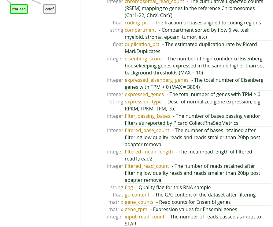
We see that gene expression data is kept in the
gene_tpm attribute. Since it is a matrix keyed to Ensembl gene
ids, we will need to find the Ensembl ids (not Hugo names) of the genes we are
interested in. For this example, we will simply use the first three options:
ENSG00000000003,ENSG00000000005,ENSG00000000419
Because we are only interested in exploring the stroma compartment, we will
also have to use the compartment attribute to narrow down our
results.
Looking at the above criteria, it seems like our research question might be formulated along the lines of:
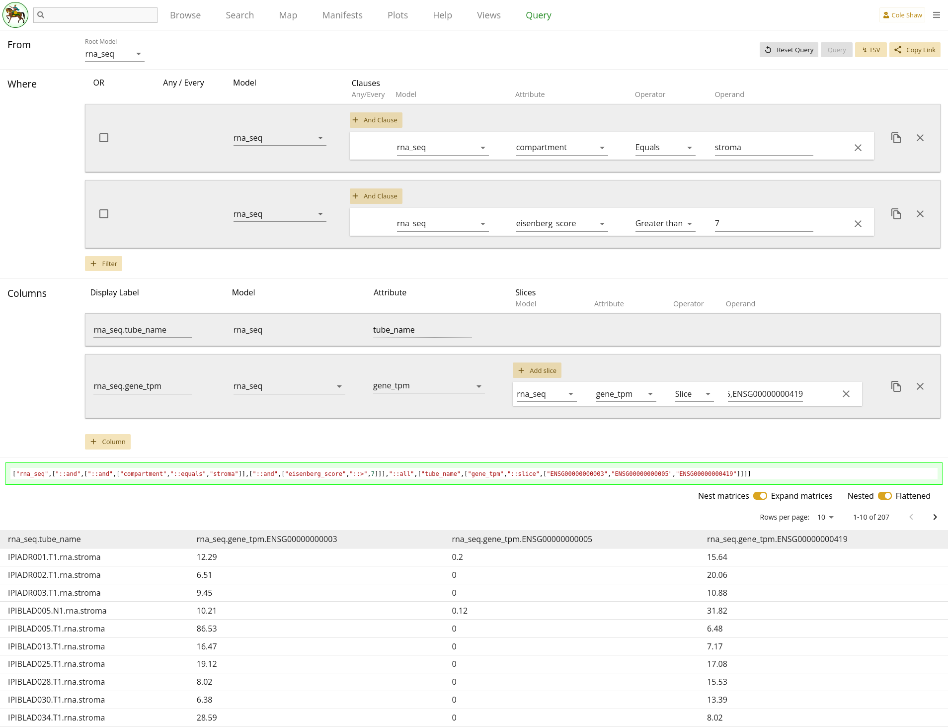
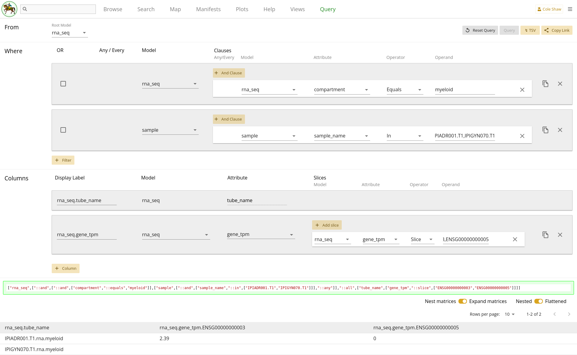
From the rna_seq model, I want the gene_tpm data for genes ENSG00000000003, ENSG00000000005, and ENSG00000000419, but only in the stroma compartment and with an eisenberg_score greater than 7 (since someone told me that 7 is a good cutoff).UI Input
Let’s translate the general question we’ve formulated into the Query UI.
From the rna_seq modelindicates that the root model should be rna_seq.
I want the gene_tpm data for genes ENSG00000000003, ENSG00000000005, and ENSG00000000419,
becomes a column, where the model is rna_seq and the attribute is
gene_tpm. Because we want only a subset of the gene data, we’ll
add a slice with the operand of
ENSG00000000003,ENSG00000000005,ENSG00000000419Lastly,
but only in the stroma compartment and with an eisenberg_score greater than 7could become two different filters. They would have the following settings:
| Filter Model | Clause Model | Attribute | Operator | Operand |
|---|---|---|---|---|
| rna_seq | rna_seq | compartment | Equals | stroma |
| rna_seq | rna_seq | eisenberg_score | Greater than | 7 |
Note that in this case, you could also create a single filter with two clauses:
| Filter Model | Clause Model | Attribute | Operator | Operand |
|---|---|---|---|---|
| rna_seq | rna_seq | compartment | Equals | stroma |
| rna_seq | eisenberg_score | Greater than | 7 |
The entire query configuration can be seen in 2.2. Now hit Query!
View in browser
You can click here to open this query in your browser, if you have access to this project.
Data Frame
You should see the first page of data in your browser, and can check out other pages or download the full data set.
Gene expression from RNA Seq, multiple compartments
Question
We are interested in exploring the expression of Progranulin from Bulk RNA Seq data in the IPI data set, specifically for the T cell and Myeloid compartments. We want to see if they are well expressed or not, so we want to see the expression value across all records regardless of quality score.
Models
From the IPI Map view, we can see that there is a model called
rna_seq, so this seems like a good place to start. If you want to
re-familiarize yourself with the model, you can check out 2.1.
Recall that gene expression data is kept in the
gene_tpm attribute. Since it is a matrix keyed to Ensembl gene
ids, we will need to find the Ensembl id for Progranulin. From the Uniprot website, we find that the Ensembl id for Progranulin is
ENSG00000030582.
Because we are only interested in exploring the T cell and myeloid
compartments, we will also have to use the compartment attribute
to narrow down our results.
Looking at the above criteria, it seems like our research question might be formulated along the lines of:
From the rna_seq model, I want the gene_tpm data for gene ENSG00000030582, but only in the tcell and myeloid compartments.UI Input
Let’s translate the general question we’ve formulated into the Query UI.
From the rna_seq modelindicates that the root model should be rna_seq.
I want the gene_tpm data for gene ENSG00000030582
becomes a column, where the model is rna_seq and the attribute is
gene_tpm. Because we want only a subset of the gene data, we’ll
add a slice with the operand of
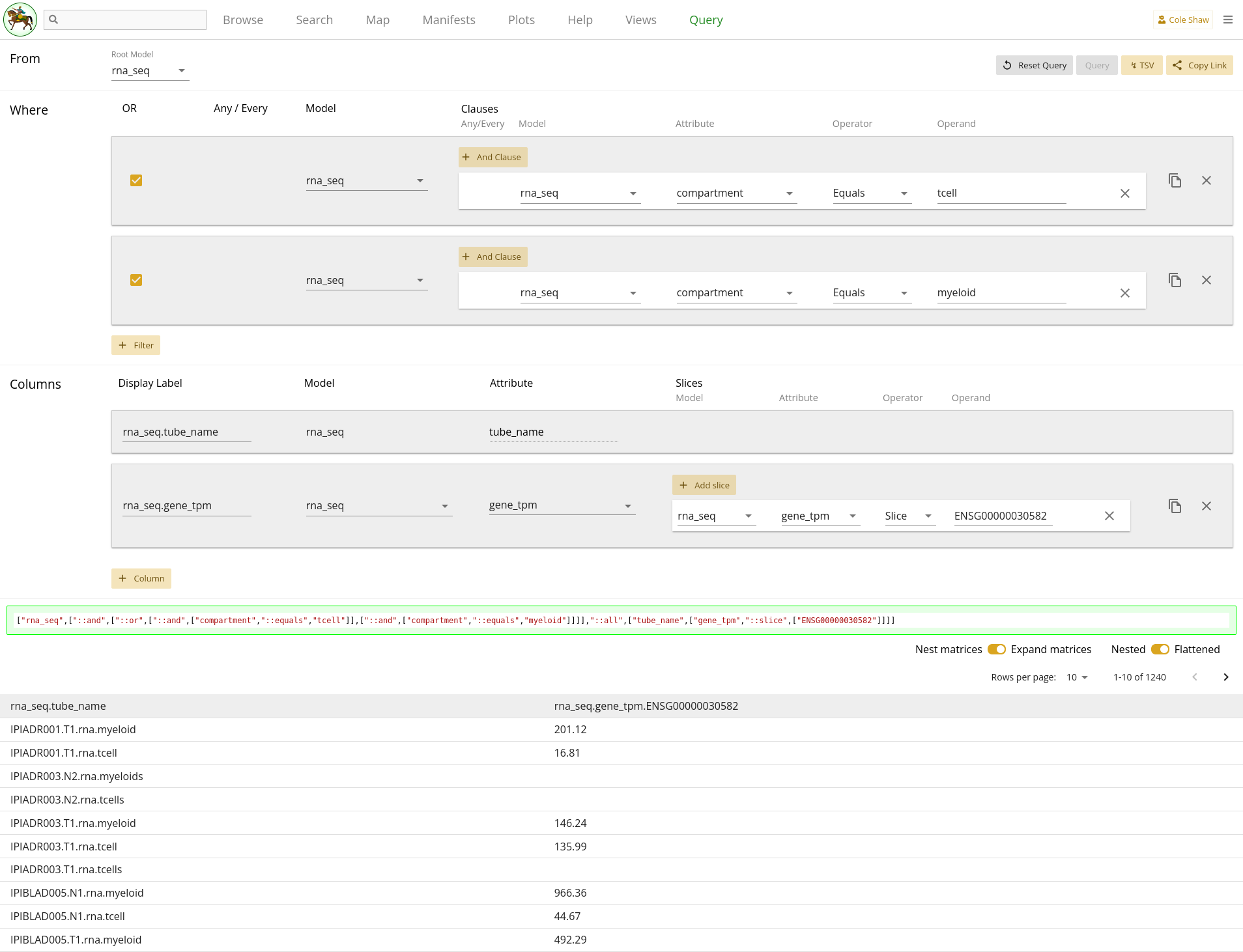
ENSG00000030582Lastly,
but only in the tcell and myeloid compartments
can be implemented in a couple of ways, both of which result in the same data
set. One way would be to use an In operator, like in 2.3.
| Filter Model | Clause Model | Attribute | Operator | Operand |
|---|---|---|---|---|
| rna_seq | rna_seq | compartment | In | tcell,myeloid |
Another way to think about the filtering is to create two separate filters, but join them with an "OR" operator. This would look like 2.4.
| Filter Model | Clause Model | Attribute | Operator | Operand |
|---|---|---|---|---|
| rna_seq | rna_seq | compartment | Equals | tcell |
| rna_seq | rna_seq | compartment | Equals | myeloid |
In the latter case, we need to make sure to check the OR checkboxes.
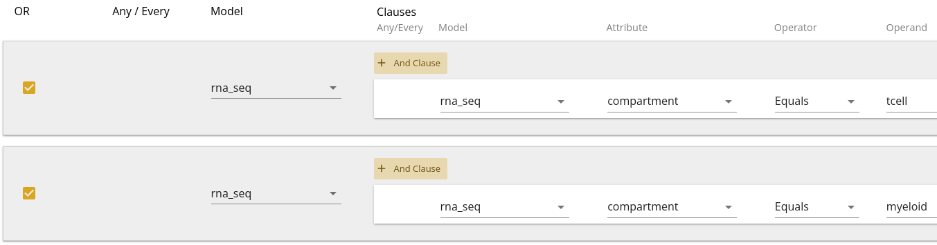
The entire query configuration can be seen in 2.4. Now hit Query!
View in browser
You can click here to open this query in your browser, if you have access to this project.
Data Frame
You should see the first page of data in your browser, and can check out other pages or download the full data set.
Note that records with no gene expression data will have blank data in the
data frame. To remove such blank fields, we could also add a filter on
rna_seq model where gene_tpm "Is Present".
Expanding on this query
Note that the compartment is included in record names for this IPI data, but
we might also wish to add a separate column with the
rna_seq model’s compartment attribute, in order to
make this easier to parse in our data frame.
Gene expression from RNA Seq, specific samples
Question
We are interested in exploring all of the gene expression data from Bulk RNA Seq data in the IPI data set, for a given set of samples that we’ve identified through other means.
Note, we should be patient with getting results from this kind of query, because gene expression data is very large and may take awhile to load from the server when not selecting specific genes. Also, because the full gene expression data set is so large, we shouldn’t expect it to render inside our browser. Instead, we will have to download the TSV results without previewing the entire data frame.
Models
From the IPI Map view, we can see that there is a model called
rna_seq, so this seems like a good place to start. If you want to
re-familiarize yourself with the model, you can check out 2.1.
Because we are only interested in exploring the samples that we have
pre-identified, we will use the sample attribute. Our target
sample set could be much larger in practice, but for the purpose of this
example, let’s say these are the only two samples in which we are interested:
    IPIADR001.T1
    IPIGYN070.T1
Looking at the above criteria, it seems like our research question might be formulated along the lines of:
From the rna_seq model, I want the gene_tpm data for all genes, but only for samples IPIADR001.T1 and IPIGYN070.T1.
You may notice that this query format goes "up the tree", becuase
rna_seq is a child of sample. In this example, let’s
also explore what this might look like if we go "down the tree":
From the sample model, I want the gene_tpm data for all the rna_seq records attached to samples IPIADR001.T1 and IPIGYN070.T1.Because Sample -> RnaSeq is one-to-many, this will result in nested data frames unless we slice out individual records when we construct our columns. If you follow along with the down-the-tree example, you’ll learn how to slice columns to get a flat data frame.
UI Input - up the tree
First, let’s translate the "up the tree" question we’ve formulated into the Query UI.
From the rna_seq modelindicates that the root model should be rna_seq.
I want the gene_tpm data for all genes
becomes a column, where the model is rna_seq and the attribute is
gene_tpm. We won’t add a slice, since we want all the gene
expression data.
Lastly,
but only for samples IPIADR001.T1 and IPIGYN070.T1
will be a filter on the Sample model. You’ll notice that if you select
rna_seq as the model, you don’t have the option to select a
sample attribute – for relationship attributes, you have to
select the target model, instead. So we’ll add a filter on Sample instead.
| Filter Model | Clause Model | Attribute | Operator | Operand |
|---|---|---|---|---|
| sample | sample | sample_name | In | IPIADR001.T1, |
| IPIGYN070.T1 |
As in the previous example, we could also use multiple operators joined by an
OR clause. However, with a lot of values, adding many filters manually can be
tedious, and a single filter with an In operator will be simpler.
The entire query configuration can be seen in 2.5. Now hit Query! Because we are not slicing the matrix column,
the render may take awhile and you may see a warning that the page is slowing
down your browser.
View in browser - up the tree
You can click here to open this query in your browser, if you have access to this project.
Data Frame - up the tree
You should see the first page of data in your browser, and can check out other pages or download the full data set.
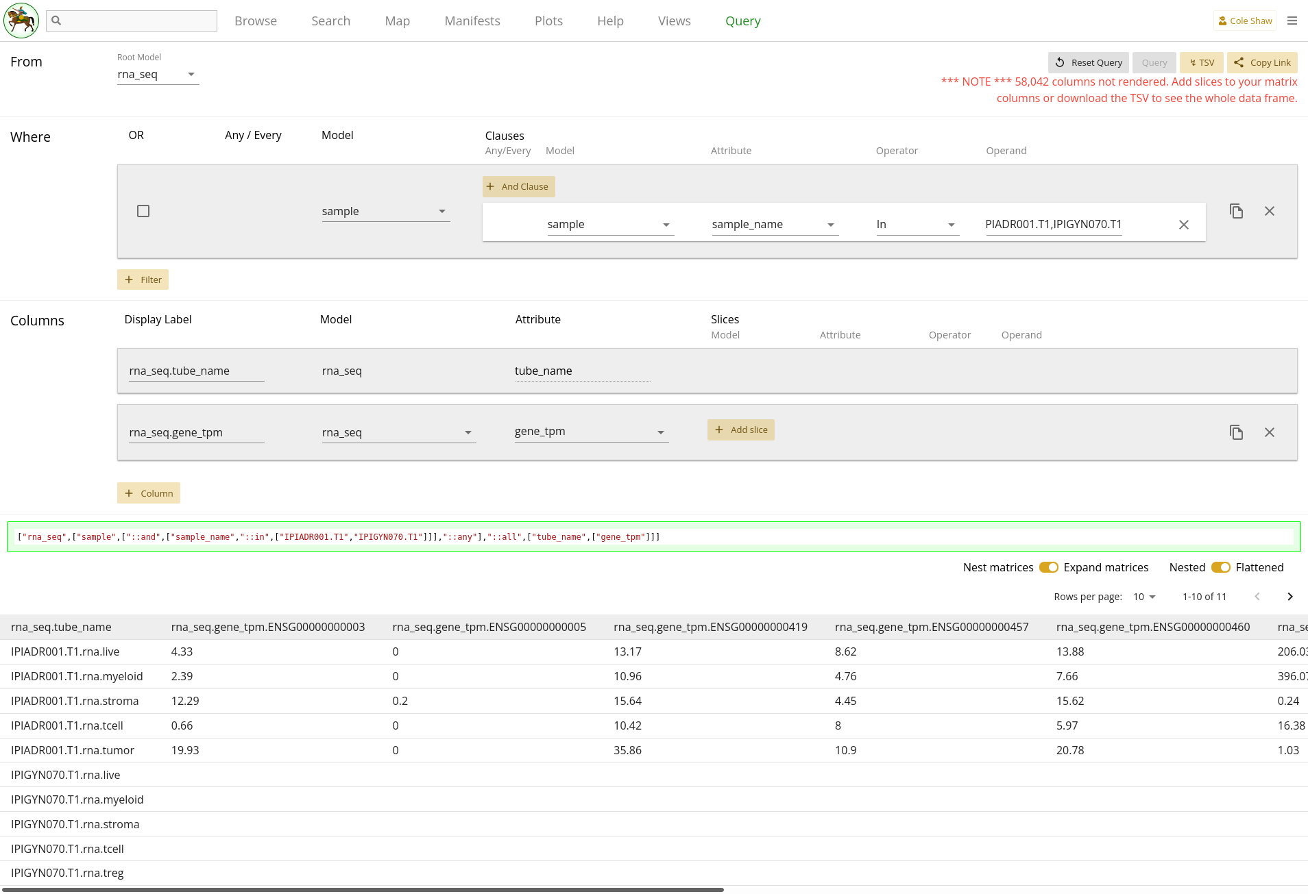
You can see that the IPIGYN070.T1 records have no gene expression
data, so just show empty values. Also, you’ll notice that because we didn’t
slice out data, all the possible gene codes are expanded, and performance is
slow. If you want the full data set, you will have to download the TSV.
Alternatively, if you know exactly the Ensembl gene ids that you want, you
should add a column slice.
UI Input - down the tree
Now let’s translate the "down the tree" question we’ve formulated for this example into the Query UI.
From the sample modelindicates that the root model should be sample.
I want the gene_tpm data for all the rna_seq records.
is actually tricky to deal with. If we do nothing else and just include the
single column, we will get nested data because there are multiple
rna_seq records attached to each of the two desired samples.
However, we don’t actually know how many rna_seq records there
are for each sample, and it’s not a consistent number of records for every
sample in the IPI data set. We can kind of guess that there should be one
record per compartment, and construct the query in that fashion, but we may
miss some data on samples with multiple rna_seq records for the
same compartment. We’ll construct this example assuming one compartment per
sample, to demonstrate how to use column slicing on collections.
There are five standard rna_seq compartments for IPI:
live
myeloid
stroma
tcell
tumor
Some samples may also have specialized compartments, like:
cd45neg
cd45pos
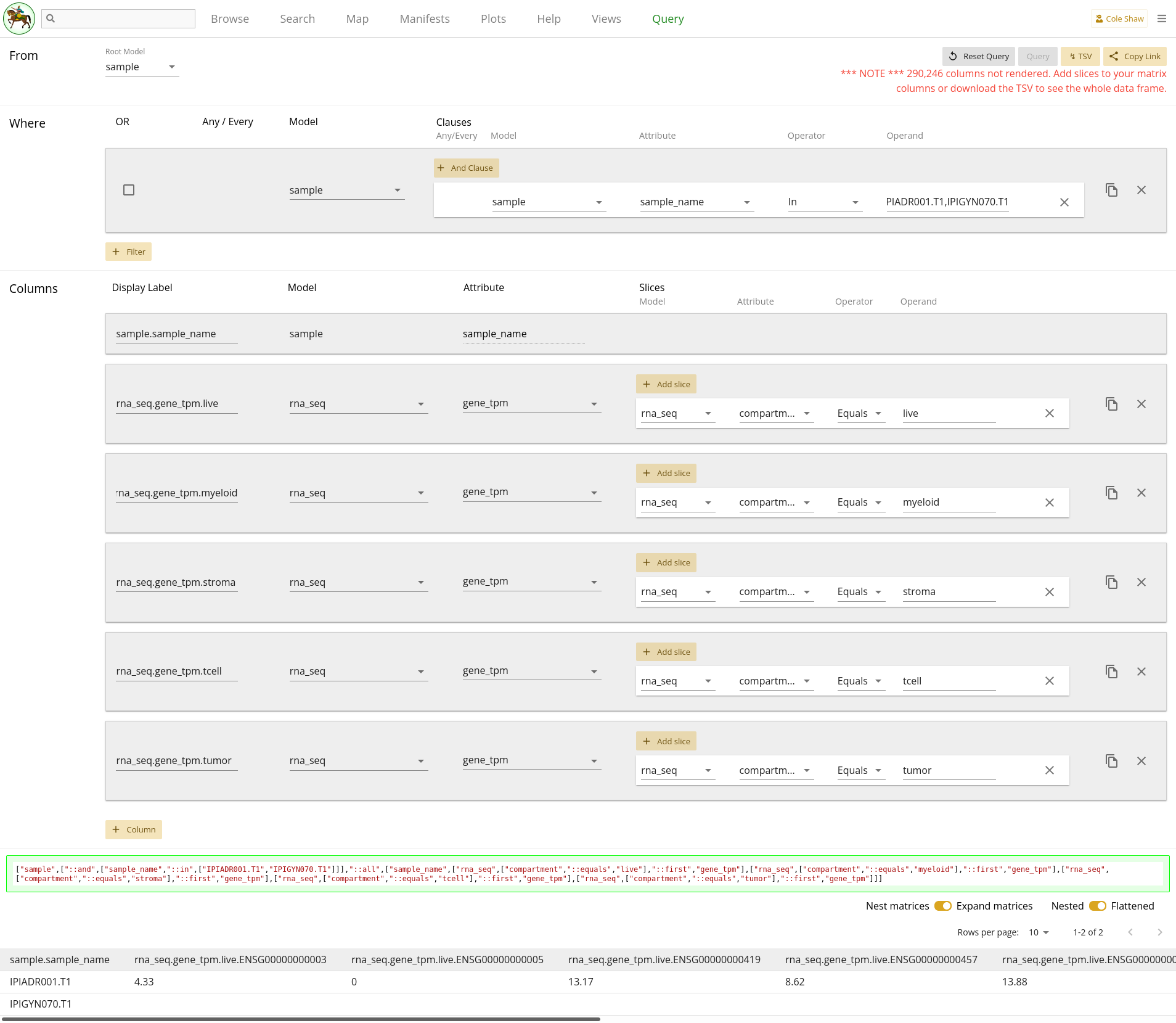
We’ll assume that the samples we’re looking at only use the five standard compartments. For each one, we’ll add a column with a slice, so we get the gene data for the "first" record of the given compartment (if there happen to be multiple). The columns would all be:
| Model | Attribute |
|---|---|
| rna_seq | gene_tpm |
| rna_seq | gene_tpm |
| rna_seq | gene_tpm |
| rna_seq | gene_tpm |
| rna_seq | gene_tpm |
With one slice per column:
| Model | Attribute | Operator | Operand |
|---|---|---|---|
| rna_seq | compartment | Equals | live |
| rna_seq | compartment | Equals | myeloid |
| rna_seq | compartment | Equals | stroma |
| rna_seq | compartment | Equals | tcell |
| rna_seq | compartment | Equals | tumor |
Because the columns are all from the same model and attribute, we’ll edit the Display Labels so we can differentiate the data in the final data frame.
Lastly,
attached to samples IPIADR001.T1 and IPIGYN070.T1
will be a filter on the Sample model’s sample_name attribute, as
in 2.5.
The entire query configuration can be seen in 2.6. Now hit Query!
View in browser - down the tree
You can click here to open this query in your browser, if you have access to this project.
Data Frame - down the tree
You should see the first page of data in your browser, though many, many columns will not be rendered, and you can check out other pages or download the full data set.
You can see that the IPIGYN070.T1 records have no gene expression
data, so just show empty values. Also, you’ll notice that because we didn’t
slice out data, all the possible gene codes are expanded, and performance is
slow (many, many columns are not rendered, as shown in the warning). If you
want the full data set, you will have to download the TSV (will be very slow).
Alternatively, if you know exactly the Ensembl gene ids that you want, you
should add a column slice.
However, if IPIADR001.T1 had multiple
live compartment records, we wouldn’t know which one was
processed for the data frame. Due to this weakness of the "down the tree"
method for this query, we would highly recommend to use the "up the tree"
method in this kind of query.
Cell populations in a collection of samples
Question
In this question, we would like to examine the frequency of CD8s vs. overall T cell population, in a collection of pre-identified samples.
Models
From the IPI Map view, we can see that there is a
model called population, so this seems like a good place to
start. You’ll note that this model is two steps away from the Sample model
(Sample -> Flow -> Population), where we have our pre-identified sample
names, so we’ll want to account for that when constructing our query.
Like the previous example, we could think about this model in "down the tree" or "up the tree" ways. Because we know that the flow data does not include any duplicate stains (each Sample has at most one flow record per stain, unlike with the Bulk RNA Seq data), we could go in either direction and extract the same data. However, because going down the tree will involve a lot of column slices, we will focus on the up the tree direction. Where relevant, we will discuss the down the tree query, as different users may find a specific approach more intuitive.
Constructing this query does assume some knowledge about how cell populations
are labelled during the flow gating process. You can use the Search page and
examine the Population model to see what names were used. For the sake of this
example, it appears that CD8a+,CD4- and
CD8a-,CD4+ may be useful population names.
To calculate total frequency of T cells, we will look for populations named
CD8a+,CD4- OR CD8a-,CD4+. We want to compare those
against the CD8 T cells, which would be populations named
CD8a+,CD4-.
Up to this point, the populations we are interested in apply regardless if we go down the tree or up the tree. If we go down the tree, we will need to add more columns and more slices for each column, to grab a single flow stain per column. If we are interested in specific stains, this could be manageable. If we are interested in all stains, this would require us to create fifteen columns for the query!! Definitely a situation where we would recommend an up-the-tree approach, with Population as the root model.
For the sake of the example, we will examine samples
IPIADR001.T1 and IPIGYN070.T1.
Looking at the above criteria and keeping to an up-the-tree query, it seems like our research question might be formulated along the lines of:
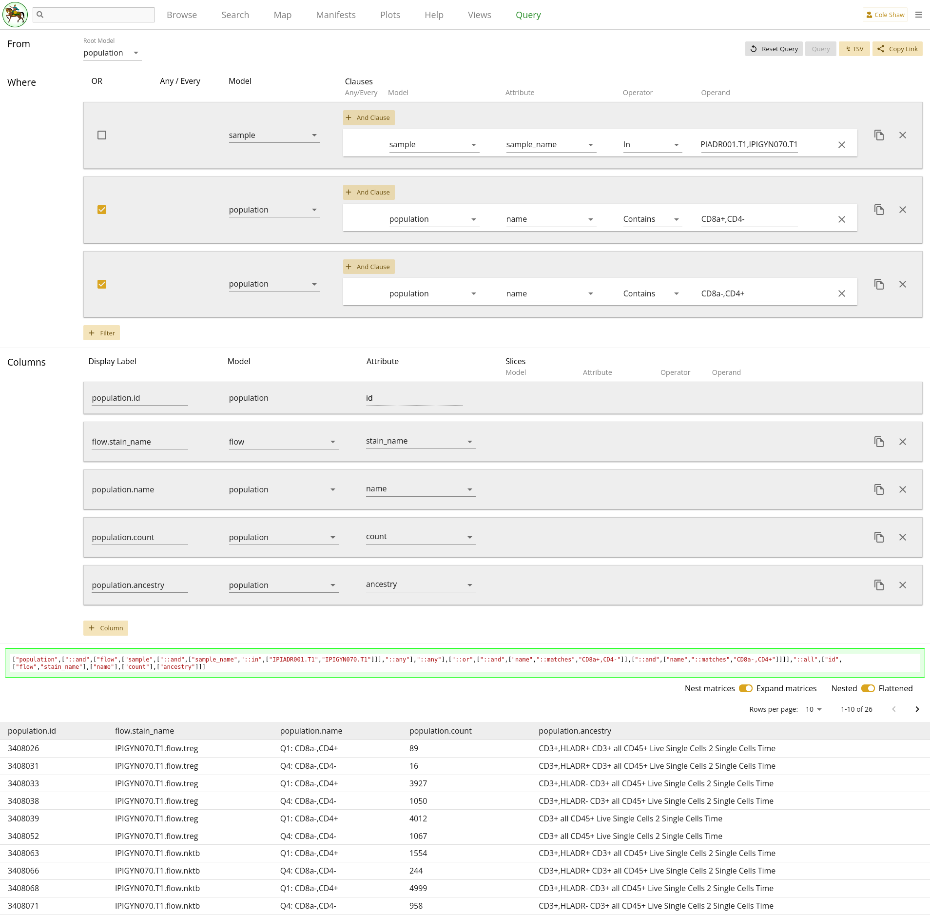
From the population model, I want the counts for the "CD8a-,CD4+" and "CD8a+,CD4-" populations, for samples IPIADR001.T1 and IPIGYN070.T1.UI Input
First, let’s translate the question we’ve formulated into the Query UI.
From the population modelindicates that the root model should be population.
I want the counts for the "CD8a-,CD4+" and "CD8a+,CD4-" populations,Since Magma itself will not perform calculations for us, we just extract the raw counts data and will have to do frequency calculations in downstream analysis.
At this point, it might seem like we should add two columns to get the two
different count values, and then perform some column slices to make sure our
data frame is flat. However, because we are using Population as the root
model, we won’t do that! Instead, we will add two filters to only pull out the
population records with those names – remember to join them with an OR clause
by checking the OR boxes. Because the population names themselves have commas,
we cannot use a single In operator in this scenario.
| Filter Model | Clause Model | Attribute | Operator | Operand |
|---|---|---|---|---|
| population | population | name | Contains | CD8a-,CD4+ |
| population | population | name | Contains | CD8a+,CD4- |
We will then add columns for name and count so that
we can separate the data and run frequency calculations in downstream
analysis. You may also decide to include ancestry and
flow stain_name if you want to gather more
information.
| Model | Attribute |
|---|---|
| population | name |
| population | count |
| population | ancestry |
| flow | stain_name |
Lastly,
for samples IPIADR001.T1 and IPIGYN070.T1will be an additional filter on the Sample model, as in 2.5.
As in the previous example, we could also use multiple operators joined by an
OR clause, for this filter instead. However, with a lot of target samples,
adding many filters manually can be tedious, and a single filter with an
In operator will be simpler.
The entire query configuration can be seen in 2.7. Now hit Query!
View in browser
You can click here to open this query in your browser, if you have access to this project.
Data Frame
You should see the first page of data in your browser, and you can check out other pages or download the full data set.
Gene expression with high T cell count
Question
In this question, we would like to extract the gene expression data in the myeloid compartment, for a given set of genes, but only for samples with a high T cell count, as assessed by flow.
Models
From the IPI Map view, we can see that both the
population (to find T cell counts) and rna_seq (to
find gene expression data) models are leaf models, and the path between them
goes through sample. However, we can note that we mainly want to
use flow population data as a filter constraint, and so perhaps we can start
with the rna_seq model as the root model, and include some Any /
Every filters.
For the sake of this example, we’ll say that we are interested in this set of genes:
ENSG00000000003,ENSG00000000005
Also, in order to construct our population filter, we will have to make some
assumptions about how populations are gated. Inspecting the Population table,
we may decide to focus on all populations named CD8a-,CD4+ OR
CD8a+,CD4-.
Looking at the above criteria, it seems like our research question might be formulated along the lines of:
From the rna_seq model, I want the gene_tpm data for ENSG00000000003 and ENSG00000000005 in the myeloid compartment, but only for samples where every flow stain has a T cell population named CD8a-,CD4+ OR CD8a+,CD4- with count greater than X.We can play around with different values of X to see what might make a good cutoff.
UI Input
First, let’s translate the question we’ve formulated into the Query UI.
From the rna_seq modelindicates that the root model should be rna_seq.
I want the gene_tpm data for ENSG00000000003 and ENSG00000000005So here we’ll add a column for gene expression data, and include a matrix slice.
| Model | Attribute | Operator | Operand |
|---|---|---|---|
| rna_seq | gene_tpm | Slice | ENSG00000000003,ENSG00000000005 |
in the myeloid compartmentSounds like a filter on rna_seq compartment!
but only for samples where every flow stain has a T cell population named CD8a-,CD4+ OR CD8a+,CD4- with count greater than XHere it definitely seems like we’ll need some additional fitlers. However, we have hit a current limitation of the Query UI, in its lack of flexibility around nesting AND and OR clauses in the filters. Ideally we would add a set of filters like
every flow stain has any population with count greater than 100 AND (name Contains CD8a-,CD4+ OR name Contains CD8a+,CD4-)
Since we cannot currently do that, we’ll break this research question up into
two distinct queries. First, we should follow the
Cell Populations example and
extract all T cell populations without any sample filters. Doing our
downstream analysis, we can determine which samples qualify as having "high T
cell count", and extract their sample IDs. At that point, we would return to
this query and add a filter on sample sample_name to
be in our set of high T cell samples (i.e. IPIADR001.T1 and
IPIGYN070.T1). This is now the same as the
Gene expression for specific samples, example! So we’ve broken up a complex query into two simpler queries. Our filters
now look like:
| Filter Model | Clause Model | Attribute | Operator | Operand |
|---|---|---|---|---|
| rna_seq | rna_seq | compartment | Equals | myeloid |
| sample | sample | sample_name | In | IPIADR001.T1, |
| IPIGYN070.T1 |
The entire query configuration can be seen in 2.8. Now hit Query!
View in browser
You can click here to open this query in your browser, if you have access to this project.
Data Frame
You should see the first page of data in your browser, and you can check out other pages or download the full data set.
HuMu
Subjects with specific assay data available
Question
Many times we want to know what data is available in the Data Library. In this case, we want to know which subjects have single cell RNA seq data available.
Models
From the HuMu Map view, we can see that there are models for
subject and sc_seq.
We might formulate our research query into:
I want to know all subject records with sc_seq data.UI Input
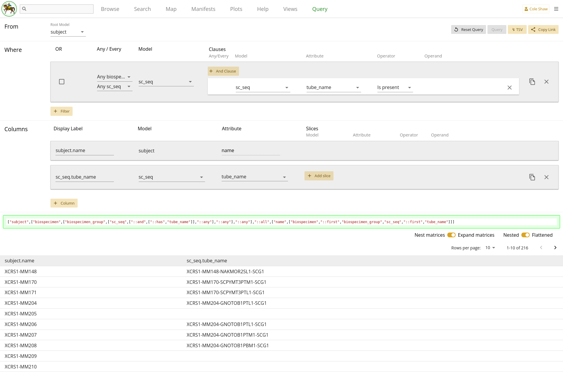
Now let’s translate the question we’ve formulated for this example into the Query UI.
I want to know all subject recordsindicates that the root model should be subject.
with sc_seq dataindicates a filter of some sort. Initially, we might be tempted to just add one like
| Filter Model | Clause Model | Attribute | operator |
|---|---|---|---|
| biospecimen_group | biospecimen_group | sc_seq | Is present |
But we’ll soon realize that we can’t construct a filter like that – the
biospecimen_group model doesn’t have an attribute option called
sc_seq. Recall that to check model data existence, we have to
perform a Is present filter on the identifier of the model
itself. So we need to add a filter like:
| Filter Model | Clause Model | Attribute | operator |
|---|---|---|---|
| sc_seq | sc_seq | tube_name | Is present |
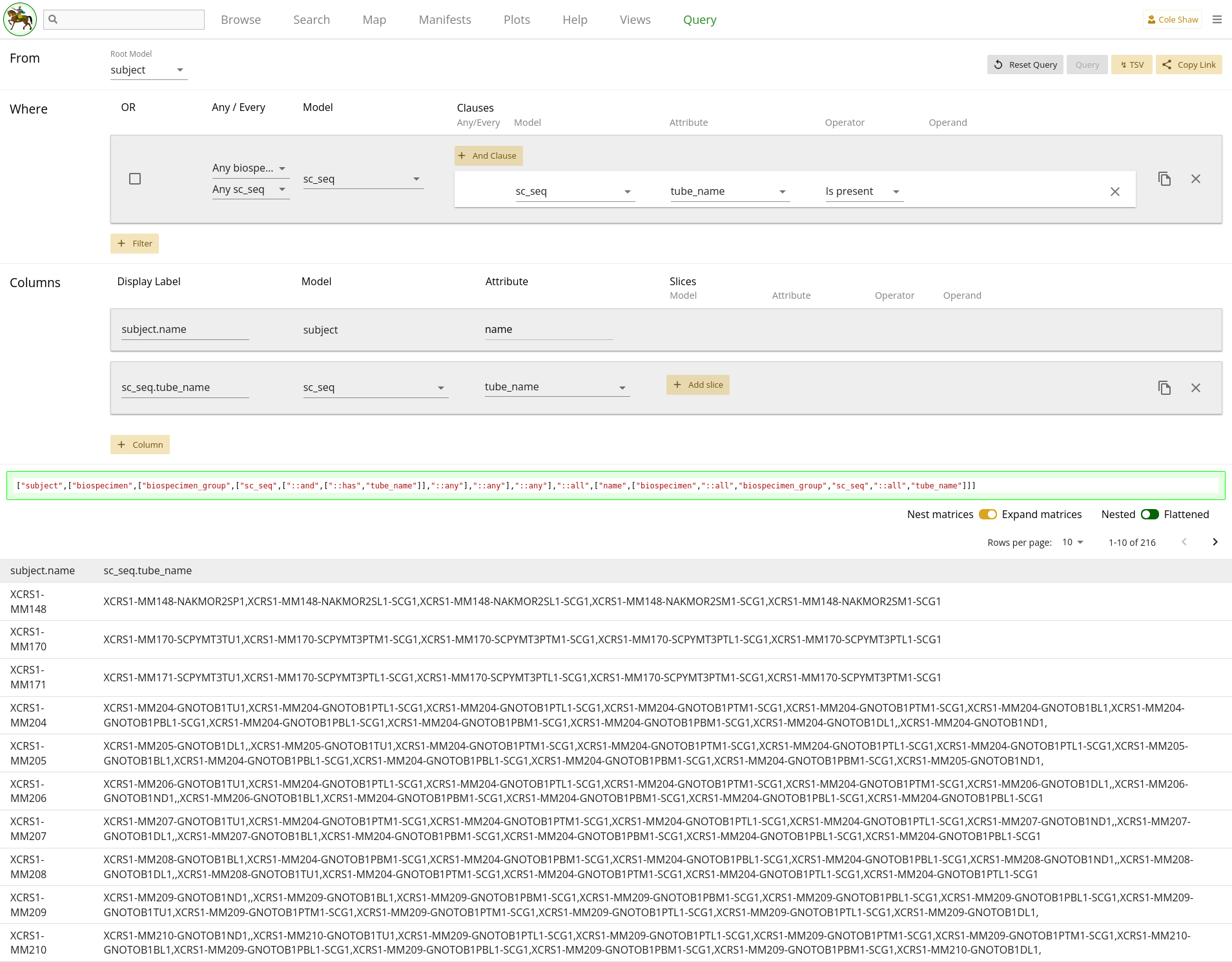
Because we want all sample records with any sort of single cell seq data, we
will leave the Any / Every toggles at Any biospecimen and
Any sc_seq.
To check our data, we’ll also add a column for the sc_seq
tube_name, so that we can more easily find the assay data.
The entire query configuration can be seen in 2.10. Now hit Query!
View in browser
You can click here to open this query in your browser, if you have access to this project.
Data Frame
Hm, it looks like the query finished, but some cells for the
tube_names are blank. What happened??!!?? How could the filter be
working (only fetch subjects with single-cell RNA seq data), yet result in no
tube_names for some subjects?
If you take a peek back at 2.9, we can see that the path from subject to
sc_seq has two one-to-many relationships. Since we did not add
any column slices, our data may not be flat! If we toggle the "Nested" vs
"Flattened" option and re-run the query, we can see that there are now data
entries in every cell.
2.10
showed blank cells because the "first" biospecimen record attached to each
subject may not have had single cell data available. By nesting, we can see
all the entries and determine if that is okay for our purposes (to gut-check
that these subjects have single cell data), or if we need to further refine
our query to get flattened data. One strategy to get flattened data might be
to set sc_seq as the root model, instead.
COMET
Analyte counts for a subset of patients
Question
For this research question, we are interested in looking at IL-6 levels for patients who have been diagnosed with COVID.
Models
From the COMET view, it may not be very intuitive where to find the IL-6 data.
However, with some digging around, we may realize that it is stored in the
analyte model.
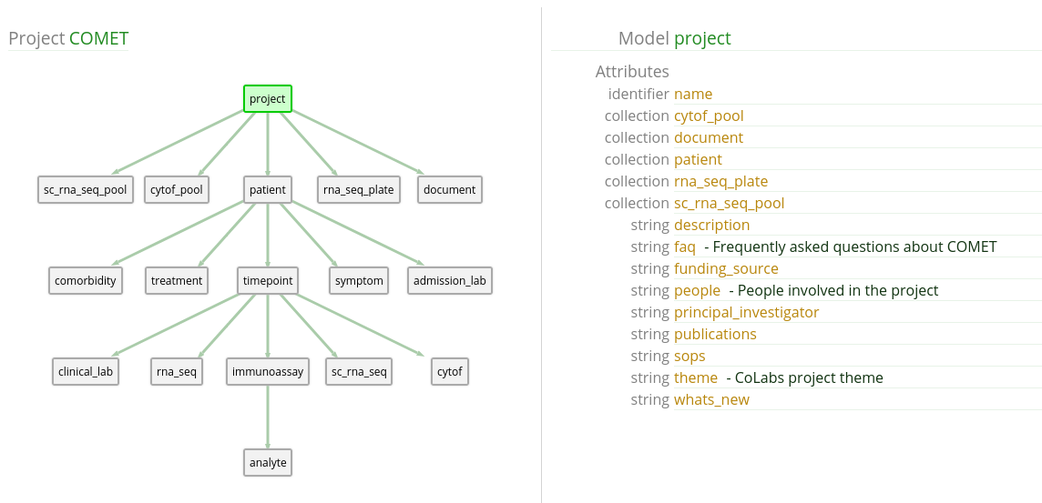
analyte has both value and
analyte_name attributes which seem like they might be useful. We
will have to examine the analyte table to know that IL-6 is
formatted as IL-6 and not something else like IL6.
Also, it looks like the patient model has an attribute that suits
our purpose, perfectly! The covid_pos boolean flag indicates
patients who have been diagnosed with COVID.
This query can be formulated in an up-the-tree fashion or down-the-tree. Let’s explore both and see what the final data frames look like. Regardless of path direction, the general research question might appear like:
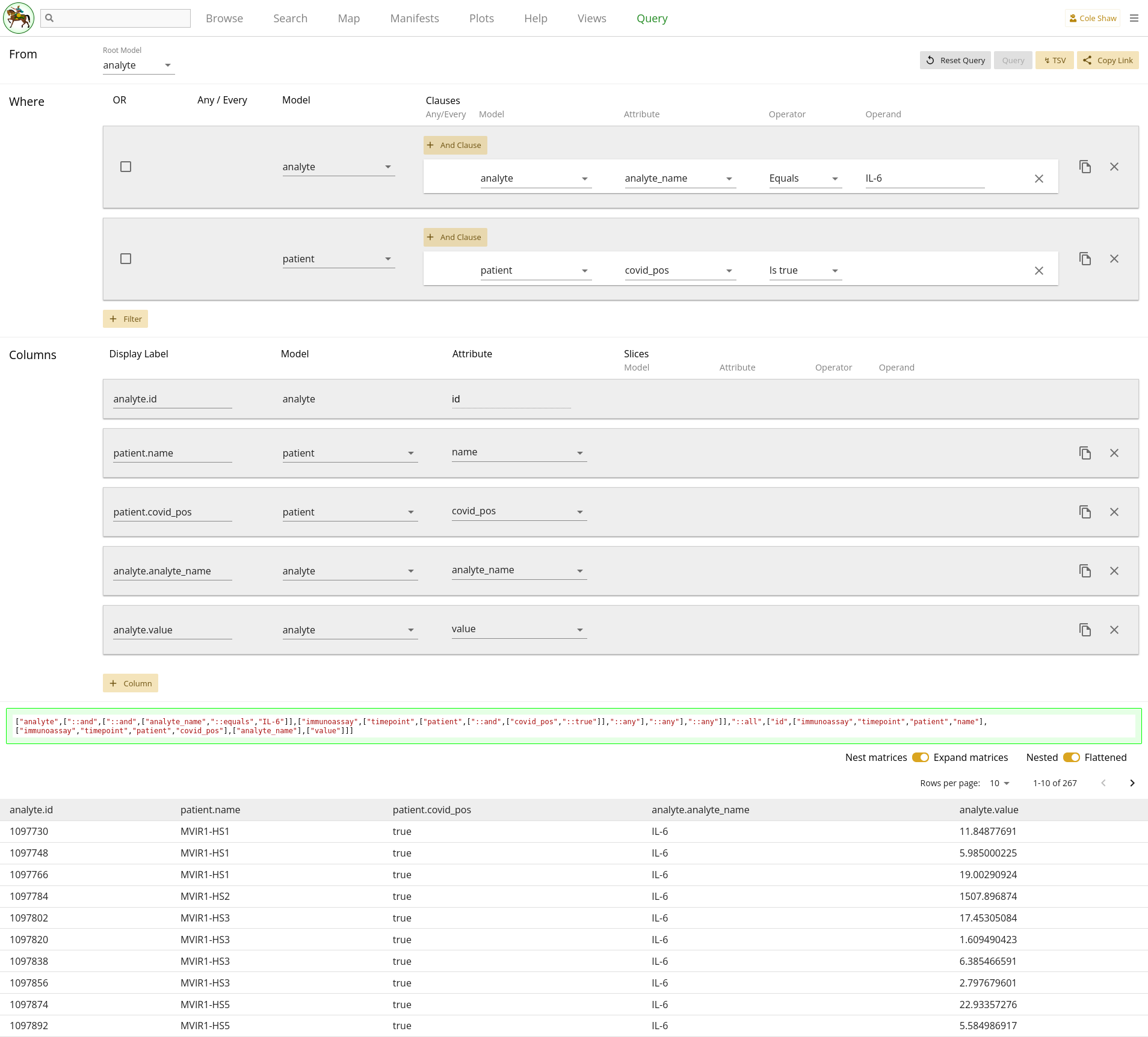
I want to know analyte value when the analyte_name is IL-6, but only for patients whose covid_pos flag is true.UI Input - up the tree
Now let’s translate the question we’ve formulated for this example into the
Query UI. Since we want to go up the tree, we’ll set the root model to
analyte.
I want to know analyte value
This is one of the output data points we want, so we’ll add a column for
analyte and attribute value.
when the analyte_name is IL-6
Because we are using analyte as the root model, this constraint
gets translated as a filter.
but only for patients whose covid_pos flag is trueWould be an additional filter, on the patient model.
| Filter Model | Clause Model | Attribute | Operator | Operand |
|---|---|---|---|---|
| analyte | analyte | analyte_name | Equals | IL-6 |
| patient | patient | covid_pos | Is true |
To check our query and give us a bit more useful context, we can also include
columns for analyte with attribute analyte_name,
patient with attribute name, and
patient with attribute covid_pos.
The entire query configuration can be seen in 2.13. Now hit Query!
View in browser - up the tree
You can click here to open this query in your browser, if you have access to this project.
Data Frame - up the tree
You should see the first page of data in your browser, and you can check out other pages or download the full data set.
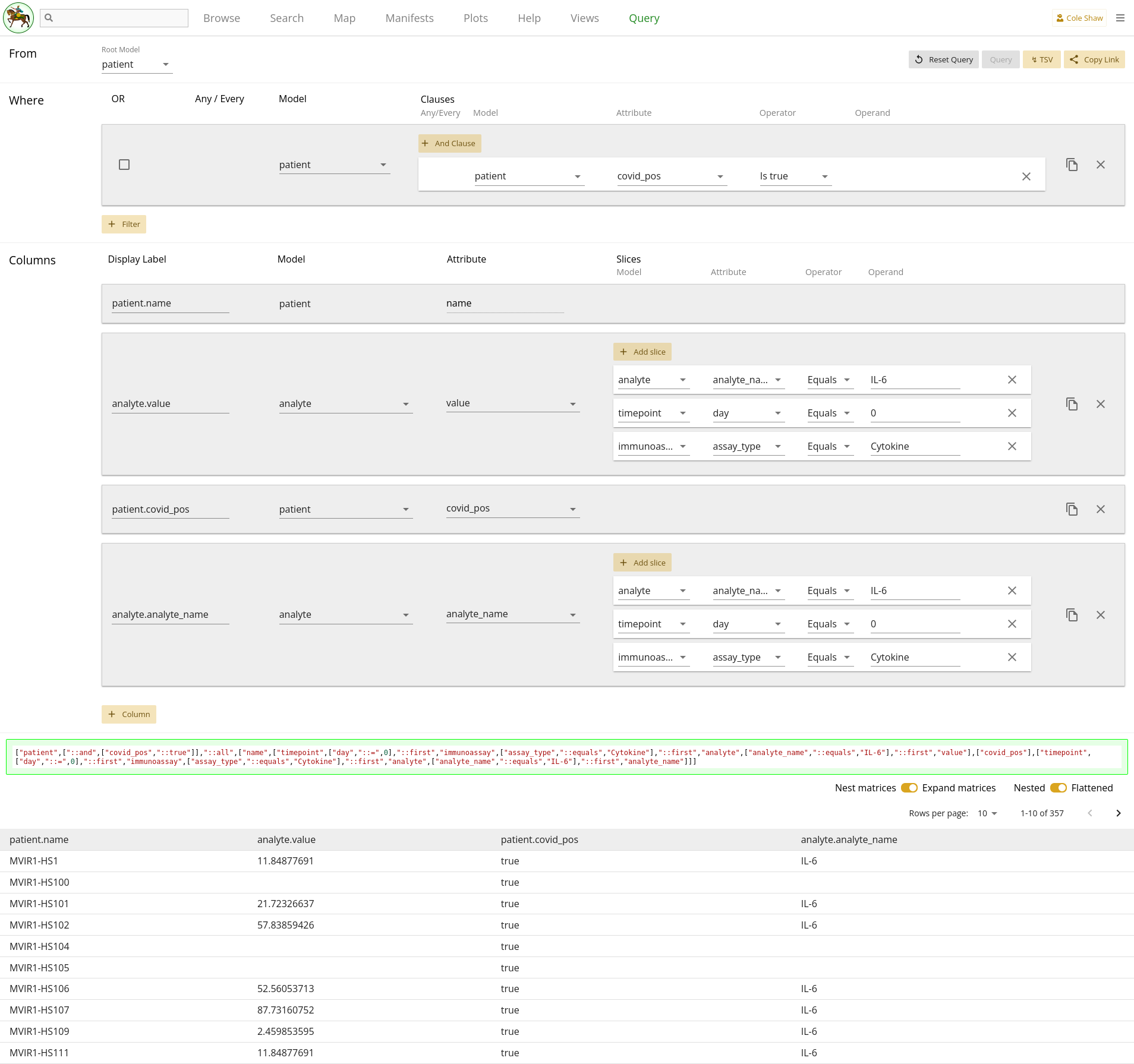
UI Input - down the tree
Now let’s translate the question we’ve formulated for this example into the
Query UI. Since we want to go down the tree, we’ll set the root model to
patient.
I want to know analyte value
This is one of the output data points we want, so we’ll add a column for
analyte and attribute value.
when the analyte_name is IL-6
Because we are using patient as the root model, this constraint
gets translated as a column slice.
| Model | Attribute | Operator | Operand |
|---|---|---|---|
| analyte | analyte_name | Equals | IL-6 |
but only for patients whose covid_pos flag is trueWould be a filter on the patient model.
| Filter Model | Clause Model | Attribute | Operator | Operand |
|---|---|---|---|---|
| patient | patient | covid_pos | Is true |
To check our query, we can also include columns for analyte with
attribute analyte_name (also slicing on
analyte_name Equals IL-6) and
patient with attribute covid_pos. The
analyte_name column with the slice is a bit superfluous, but lets
the resulting data frame look like our up-the-tree output.
The entire query configuration can be seen in 2.14. Now hit Query!
View in browser - down the tree
You can click here to open this query in your browser, if you have access to this project.
Data Frame - down the tree
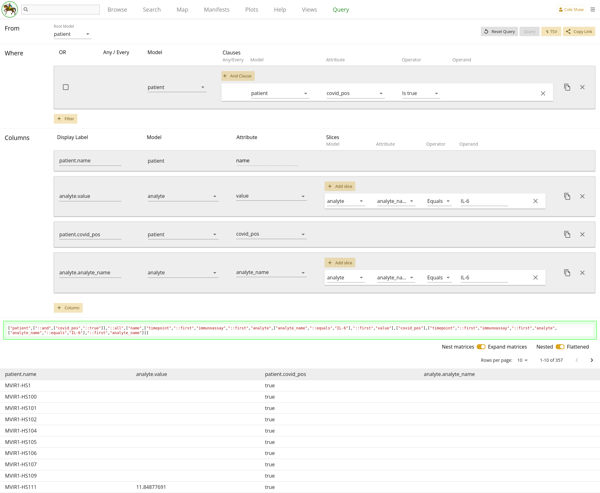
Hm...this data frame looks spectacularly blank, and doesn’t match our up-the-tree example. Let’s examine what we’ve got so far, and think about what might cause the mismatch.
Recall that down the tree paths may require column slicing, which we did for
the analyte model already. However, looking at 2.12, we can see that actually there are several one-to-many relationships along
the path of Patient -> Timepoint -> Immunoassay -> Analyte. We also
can see this by the dropdown options available in the column slice we
constructed for Analyte. Perhaps we need to add more column slices?
Adding in the right slices depends on us better understanding the COMET data
structure. Looking at the data, we may realize that each Patient has multiple
Timepoints, but cytokine data (IL-6 is a cytokine marker) was only generated
for day 0. So we should add slices for our two Analyte columns for Timepoint
where day equals 0. Also, Immunoassay appears to be fairly generic, and
different kinds of Immunoassays may have been performed on day 0 – for
example, cytokine, phip-seq, olink, etc. So we will want to also slice out
only the Immunoassay records where the assay_type equals
Cytokine. For both of our analyte columns, their
slices will then look like 2.17.
| Model | Attribute | Operator | Operand |
|---|---|---|---|
| analyte | analyte_name | Equals | IL-6 |
| timepoint | day | Equals | 0 |
| immunoassay | assay_type | Equals | Cytokine |
Querying again, we then get a data frame that better matches our up-the-tree data!
Expanding on this query
If we wanted to filter out the empty rows and get exactly the same results as up-the-tree, we could add another filter to remove those records:
| Filter Model | Clause Model | Attribute | Operator | Operand |
|---|---|---|---|---|
| analyte | analyte | analyte_name | Equals | IL-6 |
Patients with specific assay data available
Question
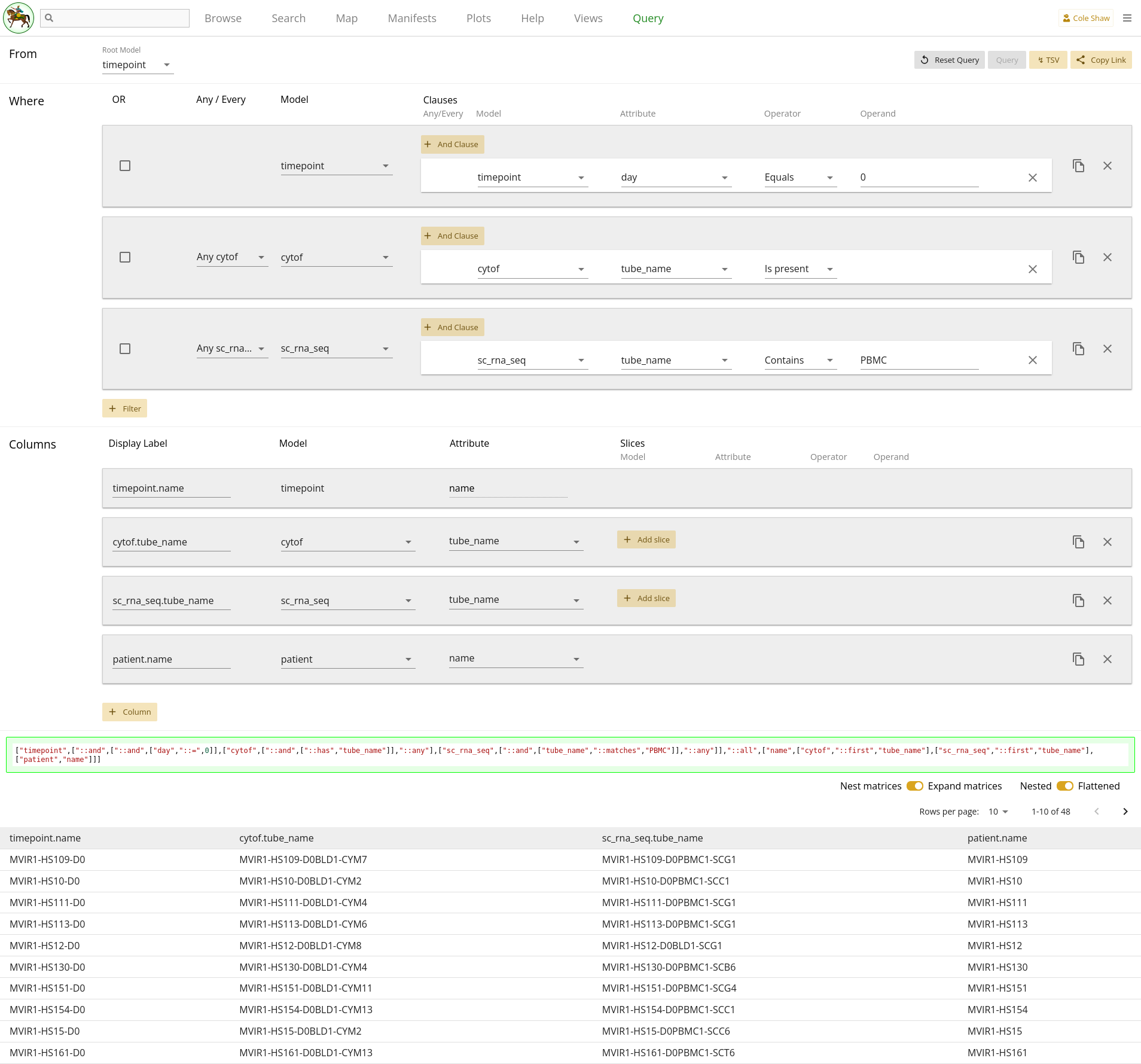
Sometimes when we are doing quality control or just want to know what is in the Data Library, we may want to do a query like, "Give me the list of patients who have X type of data". So in this example, we’ll figure out how to find the list of patients with day 0 PBMC single-cell RNA seq data as well as CyTOF data.
Models
From 2.12, we can see that both sc_rna_seq and cytof both
hang off of the timepoint model, so perhaps we should start with
timepoint as our root model.
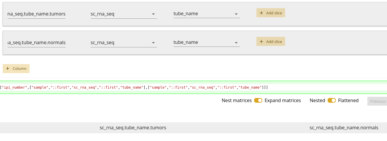
I want a list of patient names where the timepoint on day 0 has some PBMC sc_rna_seq data, as well as cytof data.UI Input
Now let’s translate the question we’ve formulated for this example into the Query UI.
I want a list of patient names
To avoid having to slice columns for Timepoint day equals 0, we’ll start with
timepoint as the root model. That means to extract the patient
name, we’ll add a column for patient, attribute
name.
where the timepoint on day 0indicates we need a filter.
has some PBMC sc_rna_seq dataAnd
as well as cytof data
Recall that to see if data exists in an assay or child collection, we add
filters that the identifier value exists for the assay model. We can find
those attributes for both models of interest from the map, and realize that
both model use tube_name as the identifier attribute.
Note that for the sc_rna_seq model, we won’t do an "exists" check
on the tube_name. Since we also want to verify that PBMC data
exists, and we know that the tube names encode the assay type, we use that
inside information to use a single filter to check for record existence plus
filter only PBMC data, instead of using two distinct filters (existence on
tube_name and match on biospecimen attribute).
So we wind up with three filters, like:
| Filter Model | Clause Model | Attribute | Operator | Operand |
|---|---|---|---|---|
| timepoint | timepoint | day | Equals | 0 |
| sc_rna_seq | sc_rna_seq | tube_name | Contains | PBMC |
| cytof | cytof | tube_name | Is present |
Because we only care that some data exists, we can leave both toggles at
Any timepoint. We can also check our query by including columns
for sc_rna_seq tube_name and cytof
tube_name.
The entire query configuration can be seen in 2.16. Now hit Query!
View in browser
You can click here to open this query in your browser, if you have access to this project.
Data Frame
You should see the first page of data in your browser, and you can check out other pages or download the full data set.
Patient data when assay data is available
Question
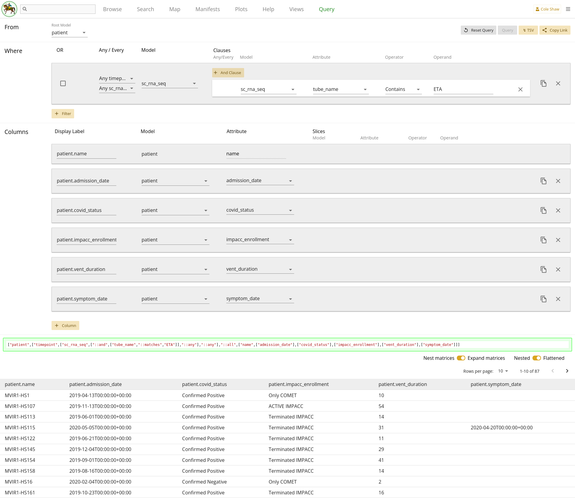
We may want to know more than just when patients have data available, like in the previous example. Sometimes we may also want to collect specific data points from a model, when assay data is available. So in this example, let’s explore a research question about grabbing a set of patient data (COVID status, IMPACC status, day enrolled, day mechanical vent, and day since symptom onset) when they have ETA single-cell RNA seq data.
Models
From 2.12, we can see that the Patient model includes the following attributes, which seem to provide the information we want:
-
covid_status -
impacc_enrollment -
admission_date -
vent_duration -
symptom_date
So we wind up with a research question that looks like:
From the patient model, I want the covid_status, impacc_enrollment, admission_date, vent_duration, and symptom_date, but only when the patient has ETA sc_rna_seq data.UI Input
Now let’s translate the question we’ve formulated for this example into the Query UI.
From the patient modelmeans we’ll set the root model as patient.
I want the covid_status, impacc\enrollment, admission_date, vent_duration, and symptom_dateindicates the set of columns that we’ll add.
but only when the patient has ETA sc_rna_seq data
will be a filter. We’ll use the same technique as in
the previous example,
where we can check that the sc_rna_seq
tube_name includes ETA to do both a data-existence
check as well as an ETA biospecimen check.
| Filter Model | Clause Model | Attribute | Operator | Operand |
|---|---|---|---|---|
| sc_rna_seq | sc_rna_seq | tube_name | Contains | ETA |
The entire query configuration can be seen in 2.17. Now hit Query!
View in browser
You can click here to open this query in your browser, if you have access to this project.
Data Frame
You should see the first page of data in your browser, and you can check out other pages or download the full data set.
Appendix
Filter operators
| Attribute Type | Operator | Operand |
|---|---|---|
| String | Contains | Yes |
| Equals | Yes | |
| Greater than | Yes | |
| Greater than or equals | Yes | |
| In | Yes | |
| Is missing | No | |
| Is present | No | |
| Less than | Yes | |
| Less than or equals | Yes | |
| Not | Yes | |
| Not in | Yes | |
| Date | Equals | Yes |
| Greater than | Yes | |
| Greater than or equals | Yes | |
| Is missing | No | |
| Is present | No | |
| Less than | Yes | |
| Less than or equals | Yes | |
| Not equals | Yes | |
| Number | Equals | Yes |
| Greater than | Yes | |
| Greater than or equals | Yes | |
| In | Yes | |
| Is missing | No | |
| Is present | No | |
| Less than | Yes | |
| Less than or equals | Yes | |
| Not equals | Yes | |
| Not in | Yes | |
| Boolean | Is false | No |
| Is missing | No | |
| Is present | No | |
| Is true | No | |
| Is untrue | No | |
| Matrix | Is missing | No |
| Is present | No |
Column slice operators
| Attribute Type | Operator | Operand |
|---|---|---|
| String | Contains | Yes |
| Equals | Yes | |
| Greater than | Yes | |
| Greater than or equals | Yes | |
| In | Yes | |
| Is missing | No | |
| Is present | No | |
| Less than | Yes | |
| Less than or equals | Yes | |
| Not | Yes | |
| Not in | Yes | |
| Date | Equals | Yes |
| Greater than | Yes | |
| Greater than or equals | Yes | |
| Is missing | No | |
| Is present | No | |
| Less than | Yes | |
| Less than or equals | Yes | |
| Not equals | Yes | |
| Number | Equals | Yes |
| Greater than | Yes | |
| Greater than or equals | Yes | |
| In | Yes | |
| Is missing | No | |
| Is present | No | |
| Less than | Yes | |
| Less than or equals | Yes | |
| Not equals | Yes | |
| Not in | Yes | |
| Boolean | Is false | No |
| Is missing | No | |
| Is present | No | |
| Is true | No | |
| Is untrue | No | |
| Matrix | Slice | Yes |